20141018 – Non-magic PLLs
I am not going to rehash the full theory of PLL’s here, there are plenty of places on the net which does that much more competently that I could ever do.
Most of them fail to tell you that a PLL is just a PI control loop with phase errors for input and frequency ajustments for output. If you look up PI control loops, you will find entirely different explanations.
(This obviously begs the question: Why not use PID control loops for timekeeping ? The answer is that we have too much noise on our phase error measurements.)
For our purposes a PLL looks like this:
double integrator = 0.0;

while (1) {
        phase_error = measure();
        integrator += phase_error * I;
        set_frequency(-(phase_error * P + integrator));
        sleep(poll_interval);
}
The only magic there is in a PLL, is picking the right I and P for the poll_interval.
If you want a good safe place to start:
P = 0.08 / poll_interval;
I = 0.30 * P * P * poll_interval;
PLL behaviour
Before we continue, lets try to get a feel for what these three parameters do.
In the next three plots, the simulated local clock is 100 PPM wrong, and the clock has no offset when the simulation starts.
First, we can vary the poll_interval:
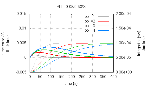
The longer the poll interval, the longer before the integrator matches the frequency error. Notice that the worst case time error also increases with longer poll interval.
Second, we can vary the P(roportional) term:
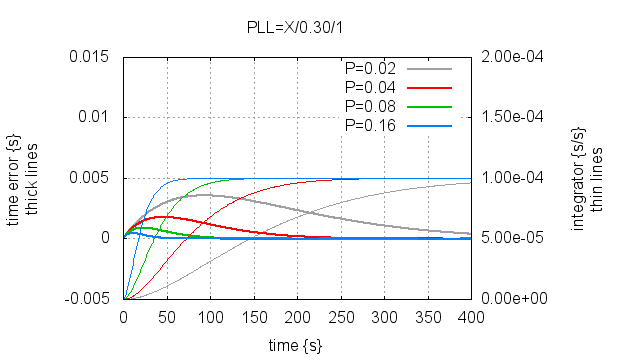
This is not too different from changing the poll interval, which is a consequence of the I(ntegral) term being defined from the P(proportional) term. Without this coupling, the PLL may oscillate rather than converge.
Finally, we can vary the I(ntegral) term:
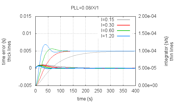
If we use a larger I term, we find the frequency faster, but this increased sensistivity also causes “overshoot” or “ringing”.
In these three examples, we used perfect phase error measurements with no noise. In practice there is noise, and if the PLL is tuned so it overshoots, this can cause instability.
If P, I and poll_interval can be chosen freely, the only limiting factor on PLL performance is the noise in the phase error measurements.
If you want to play around with this yourself, I have included below the 111 lines of python source-code which generated these three plots.
(If you think you have found a set of perfect parameters, remember to add a noise component to the second argument of the pll_code() call in the run function :-)
NTP PLLs
In an NTP context, the phase error measurement is the big problem, but it is not the only problem.
NTP servers are a finite resource, so we simply cannot have every client poll its servers once per second. Historically once ever 64 seconds is the maximum rate, and once per 1024 seconds is desirable.
But we also want clients to get “on time” really fast after startup, we don’t want to wait hours or for that matter minutes before our application can trust the timestamps from the kernel.
This calls for non-constant P, I and poll_interval, and this is where PLL design starts to get tricky.
Ideally our PLL will measure/estimate the noise on the phase error measurements, which is more or less the RTT to the server, and tune itself accordingly for the optimal startup performance, then once the local frequency error has been estimated, it will estimate the stability of the local timebase as measured against the servers presumably perfect timekeeping, and tune the PLL for the optimal long term timekeeping.
That would be a seriously magic PLL…
phk
PLL simulator sourcecode:
#!/usr/bin/env python

from __future__ import print_function

import subprocess

def run(fn, length, pll_code, freq_err = 100e-6, time_err = 10e-3):
        t = 0
        lt = time_err
        freq_adj = 0.0
        fo = open(fn, "w")
        for i in range(length):
                t += 1.0
                lt += (freq_err + freq_adj)
                err = lt
                freq_adj = pll_code(t, err, fo)
        fo.close()

def plot(fn, title, ll, yrange = "-5e-3:15e-3", y2range = "0:200e-6",
    xtics = None):
        fo = open("/tmp/_g", "w")
        fo.write("set title '%s'\n" % title)
        fo.write("set yrange [%s]\n" % yrange)
        fo.write('set ylabel "time error {s}\\nthick lines"\n')
        fo.write("set y2range [%s]\n" % y2range)
        fo.write('set y2label "integrator {s/s}\\nthin lines"\n')
        fo.write("set xlabel 'time {s}'\n")
        fo.write("set style data line\n")
        fo.write("set grid\n")

        if xtics != None:
                fo.write("set xtics %s\n" % xtics)

        fo.write("set y2tics\n")
        fo.write("set y2tics format '%.2e'\n")

        fo.write("set term png size 640,360\n")
        fo.write("set output '%s'\n" % fn)
        fo.write("plot ")
        sep = ""
        n = 0
        for i,j in ll:
                fo.write(sep + "'%s' lc %d lw 2 title '%s'" % (i, n, j))
                sep = ","
                fo.write(sep + "'%s' using 1:3 axis x1y2 lc %d lw 1 notitle" %
                    (i, n))
                n += 1
        fo.write("\n")
        fo.write("set output\n")
        fo.write("set term wxt 0\n")
        fo.close()
        subprocess.call(["gnuplot", "/tmp/_g"])

class pll(object):
        def __init__(self, cp, ci, poll):
                self.P = cp / poll
                self.I = ci * self.P * self.P * poll
                self.integ = 0.0
                self.poll = poll
                self.counter = 0
                self.freq_adj = 0.0

        def pll(self, tim, err, fo):
                self.counter += 1
                if self.counter < self.poll:
                        return -self.freq_adj
                self.counter = 0
                self.integ += self.I * err
                self.freq_adj = self.P * err + self.integ
                fo.write("%4d %.3e %.3e %.3e\n" %
                    (tim, err, self.integ, self.freq_adj))
                return -self.freq_adj

#######################################################################
run("/tmp/_s1",  400, pll(0.08, 0.30, 1).pll, time_err = 0)
run("/tmp/_s2",  400, pll(0.08, 0.30, 2).pll, time_err = 0)
run("/tmp/_s3",  400, pll(0.08, 0.30, 3).pll, time_err = 0)
run("/tmp/_s4",  400, pll(0.08, 0.30, 4).pll, time_err = 0)

plot("20141018_fig1.png", "PLL=0.08/0.30/X", [
        [ "/tmp/_s1", "poll=1" ],
        [ "/tmp/_s2", "poll=2" ],
        [ "/tmp/_s3", "poll=3" ],
        [ "/tmp/_s4", "poll=4" ],
])

#######################################################################
run("/tmp/_s1",  400, pll(0.02, 0.30, 1).pll, time_err = 0)
run("/tmp/_s2",  400, pll(0.04, 0.30, 1).pll, time_err = 0)
run("/tmp/_s3",  400, pll(0.08, 0.30, 1).pll, time_err = 0)
run("/tmp/_s4",  400, pll(0.16, 0.30, 1).pll, time_err = 0)

plot("20141018_fig2.png", "PLL=X/0.30/1", [
        [ "/tmp/_s1", "P=0.02" ],
        [ "/tmp/_s2", "P=0.04" ],
        [ "/tmp/_s3", "P=0.08" ],
        [ "/tmp/_s4", "P=0.16" ],
])

#######################################################################
run("/tmp/_s1",  400, pll(0.08, 0.15, 1).pll, time_err = 0)
run("/tmp/_s2",  400, pll(0.08, 0.30, 1).pll, time_err = 0)
run("/tmp/_s3",  400, pll(0.08, 0.60, 1).pll, time_err = 0)
run("/tmp/_s4",  400, pll(0.08, 1.20, 1).pll, time_err = 0)

plot("20141018_fig3.png", "PLL=0.08/X/1", [
        [ "/tmp/_s1", "I=0.15" ],
        [ "/tmp/_s2", "I=0.30" ],
        [ "/tmp/_s3", "I=0.60" ],
        [ "/tmp/_s4", "I=1.20" ],
])
phk